Convolutional Sequence to Sequence Learning - 2017

Information

Link: Arxiv

Paper by: Facebook AI Research (FAIR)

Why is this paper important?: Introduced convolution operations for sequence to sequence problems.

Code: Fairseq - Facebook Research

Summary

This paper tackles sequence to sequence problems such as Machine Translation (MT) and Abstractive Summarization by applying convolutional layers.

Input

Start with \(\textbf{x}\) which is the input sequence that is tokenized (by classical space-separation, Byte-Pair Encoding or Wordpiece etc.):

\[\textbf{x} = (x_{1}, . . . , x_{m})\]

where \(x_{1}\) would correspond to the first token.

All of these tokens are embedded in distributional space as

\[\textbf{w} = (w_{1}, . . . , w_{m})\]

where \(w_{1}\) corresponds to the embedding of the first token (\(x_{1}\)).

These \(w_{i}\)’s have dimension of \(\mathcal{R}^{f}\) and are retrieved from a matrix \(D \in \mathcal{R}^{V \times f}\) which is the embedding matrix.

To give the model a sense of the positions of the input tokens, we add absolute position embeddings to each of the token embeddings. Position embeddings:

\[\textbf{p} = (p_{1}, . . . , p_{m})\]

where \(p_{1}\) corresponds to the absolute position embedding of the first token (\(x_{1}\)) and has a dimension \(\mathcal{R}^{f}\).

Then combine all token embeddings (\(w_{i}\)) with absolute position embeddings by element-wise adding each vector pair to construct final representations of the input tokens:

\[\textbf{e} = (w_{1} + p_{1}, . . . , w_{m} + p_{m})\]

Encoder

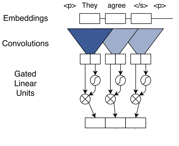
Each convolution kernel in the encoder takes \(k\) input elements (\(e_{i}\)) concatenated together. The output from this computation is \(A\). We use another convolutional kernel to produce another vector (with the same dimension as \(A\)): \(B\). Then this \(B\) is put through a non-linearity which is a Gated Linear Unit (GLU) in the paper. Then \(A\) is element-wise multiplied with the output from the GLU: \(\sigma (B)\)

\[v([A B]) = A \otimes \sigma (B)\]

The computations till now can be diagrammed as below:

Figure 1 - Encoder (without the Residual Connection)

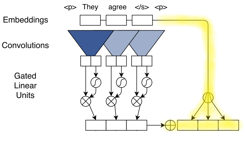
There are also residual connections from the input to the output of each convolutional block (convolution + nonlinearity). This enables gradient propagation through a large number of layers:

\[z_{i}^{l} = v(W^{l} [ z_{i-k/2}^{l-1}, ... , z_{i+k/2}^{l-1} ] + b_{w}^{l}) + z_{i}^{l-1}\]

where \(v(...)\) represents the convolution + nonlinearity operation done on the previous layer’s or input’s concatenated vectors and \(z_{i}^{l-1}\) represents the single vector output from the previous layer. In the paper, the residual connection is highlighted here:

Figure 2 - Residual Connection in Encoder

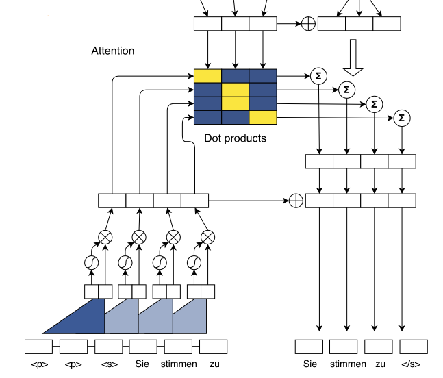
Multi-step Attention

The architecture uses separate attention mechanisms for each decoder layer.

\[d_{i}^{l} = W_{d}^{l}h_{i}^{l} + b_{d}^{l} + g_{i}\]

where \(h_{i}^{l}\) is the current decoder state and \(g_{i}\) is the embedding of the previous target token. And the attention of state \(i\) and source token \(j\) is:

\[a_{ij}^{l} = \frac{exp(d_{i}^{l} \cdot z_{j}^{u})}{\sum_{t=1}^{m} exp(d_{i}^{l} \cdot z_{t}^{u})}\] \[c_{i}^{l} = \sum_{j=1}^{m} a_{ij}^{l}(z_{l}^{u} + e_{j})\]

where \(c_{i}^{l}\) is the conditional input to the current decoder layer.

Figure 3 - Multi-step Attention

Decoder

After the last layer of the decoder, a distribution is computed over the T (=target vocabulary size) possible target token \(y_{i+1}\) by:

\[p(y_{i+1}|y_{1},...,y_{i}, \textbf{x}) = softmax(W_{o}h_{i}^{L} + b_{o})\]

Datasets

• Translation
  • WMT’16 English-Romanian
  • WMT’14 English-German
  • WMT’14 English-French
• Summarization (Abstractive)
  • Gigaword
  • DUC-2004